Using Thermodynamic Descriptors
The previous tutorials have explained how to create a kinetic model which uses binding energies of key intermediates as “descriptors” in order to create a “map” of catalytic activity across different types of surfaces. This type of analysis is useful for catalyst screening, but it is also often interesting to take a closer look at a single catalyst surface and explore the effect of reaction conditions. In order to do this in CatMAP we will use the same framework as discussed in the Code Overview. The only difference is that instead of using energies as descriptors we will use “thermodynamic variables” (temperature, pressure for now) as descriptors. Naturally this also means that we will need to use a different “scaler” which, instead of creating a linear map uses some pre-defined expressions to add in the proper free energy contributions.
To make this clearer we will continue with the CO oxidation example and examine CO oxidation on Pt(111) as a function of temperature and pressure. Again, the purpose is not to make a publishable analysis but to become familiar with the functionality of CatMAP. We will be able to use a “submission script” (mkm_job.py) very similar to the one from Refining a Microkinetic Model.
from catmap import ReactionModel

mkm_file = 'CO_oxidation.mkm'
model = ReactionModel(setup_file=mkm_file)
model.output_variables += ['production_rate']
model.run()

from catmap import analyze

vm = analyze.VectorMap(model)
vm.plot_variable = 'production_rate' #tell the model which output to plot
vm.log_scale = True #rates should be plotted on a log-scale
vm.min = 1e-25 #minimum rate to plot
vm.max = 1e3 #maximum rate to plot
vm.threshold = 1e-25 #anything below this is considered to be 0
vm.subplots_adjust_kwargs = {'left':0.2,'right':0.8,'bottom':0.15}
vm.plot(save='production_rate.pdf')
For simplicity we will only look at the “production_rate” output variable in this tutorial. Other outputs can be calculated/analyzed as described in tutorials 2-3, Creating a Microkinetic Model and Refining a Microkinetic Model.
We will use a reaction model similar to the simple one used in Creating a Microkinetic Model since this will run faster than the more complicated models. In order to refine this to something more sophisticated you can follow the strategy outlined in Refining a Microkinetic Model. This also means that we can re-use the energies.txt file from Creating a Microkinetic Model, although we can make it even shorter since we only care about the Pt(111) energies:
surface_name        site_name       species_name    formation_energy        bulk_structure  frequencies     other_parameters        reference
None        gas     CO2     2.45    None    [1333,2349,667,667]     []      "Angew. Chem. Int. Ed., 47, 4835 (2008)"
None        gas     CO      2.74    None    [2170]  []      "Energy Environ. Sci., 3, 1311-1315 (2010)"
None        gas     O2      5.42    None    [1580]  []      Falsig et al (2012)
Pt  111     O       1.62    fcc     []      []      Falsig et al (2012)
Pt  111     CO      1.7     fcc     []      []      "Angew. Chem. Int. Ed., 47, 4835 (2008)"
Pt  111     O-CO    4.04    fcc     []      []      "Angew. Chem. Int. Ed., 47, 4835 (2008)"
Pt  111     O-O     5.35    fcc     []      []      Falsig et al (2012)
Note that we could also leave all the other energies in since the parser will just ignore any lines it doesn’t need. Finally, there is the “setup file” - CO_oxidation.mkm. This is where all of the necessary changes must be made in order to use “thermodynamic descriptors”. We will start with the same setup file from Creating a Microkinetic Model, but we need to make the following changes:
Change the scaler Add the following line somewhere in the setup file (usually near the beginning):
scaler = 'ThermodynamicScaler'As you can probably guess this tells CatMAP to use the “ThermodynamicScaler” class to move from “descriptor space” to “parameter space” (see Code Overview). This class will use whatever “thermo modes” are defined for gas phase/adsorbate species in order to add free energy contributions (see Creating a Microkinetic Model).Choose the relevant surface Next we need to tell CatMAP which surface to use. For this example we will look at Pt(111). To do this we just need to change the “surface_names” variable:
surface_names = ['Pt']
Note that the (111) surface is already selected due to the line:
species_definitions['s'] = {'site_names': ['111'], 'total':1}
Change the descriptors Now we need to tell the “ThermodynamicScaler” which two variables we will be using for descriptors, and we need to modify the ranges over which to vary these descriptors. Currently only temperature and pressure are implemented, although there is also an option to use log(pressure) as discussed later. For now lets look at temperatures from 400 - 1000 K and pressures from 1e-8 to 1000 bar:
descriptor_names= ['temperature','pressure']
descriptor_ranges = [[400,1000],[1e-8,1e3]]
Modify temperature/pressure to be compatible - In Creating a Microkinetic Model we used a model where temperature and pressure were explicitly specified. This doesn’t really make sense now, since we are varying these two variables. The temperature ends up not really mattering since it will be over-written as CatMAP moves through descriptor space; however, just to be unambiguous its good practice to delete the following line:
temperature = 500 #Temperature of the reaction
Finally, we need to tell CatMAP how to handle the pressures. Previously we just defined “static pressures” for each gas-phase species, but that doesn’t make sense if the total pressure is varying. In order to get around this we instead specify “concentrations” for each gas-phase species:
species_definitions['CO_g'] = {'concentration':2./3.}
species_definitions['O2_g'] = {'concentration':1./3.}
species_definitions['CO2_g'] = {'concentration':0}
Note that this “concentration” is not normalized - the total pressure of a gas at any total pressure will be given by concentration*P where P is the total pressure. Thus, if the concentrations do not sum to 1 then the “pressure” axis will be incorrect.
After making these changes we can run the “submission script” with:
sh python mkm_job.py
which should give the usual kind of output. When it finishes you should see the following “production_rate.pdf” in the folder:
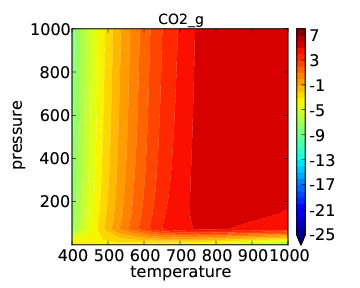
As expected, the temperature dependence is much more drastic than the pressure dependence. In many cases it makes more sense to look at pressure dependence on a log scale. This is easily achieved by changing the descriptor names/ranges:
descriptor_names= ['temperature','logPressure']
descriptor_ranges = [[400,1000],[-8,3]]
Note that the “log” in this notation refers to a base 10 logarithm so that the plot produced is the same as before, but with pressure on a log scale. If we now run the submission script we get the following output:
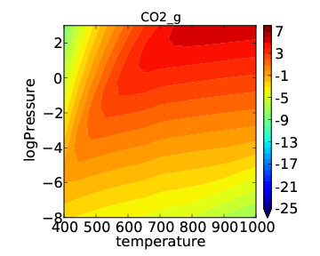
This looks a little nicer than the previous plot since the low pressure behavior has higher resolution.
We can see from this tutorial that it is fairly easy to move between a micro-kinetic model for a screening study and one for a “reaction condition” study (and vice-versa). Only a few lines of the “setup file” need to be changed. This is one advantage of CatMAP - once you setup a reaction model once you can re-use it for several different analyses.