Creating a Microkinetic Model
This tutorial provides a walk-through of how to create a very basic micro-kinetic model for CO oxidation on transition-metal (111) surfaces. More advanced features are explored in Refining a Microkinetic Model and the Topics section.
Setting up the model
All micro-kinetic models require a minimum of 2 files: the “setup file” and the “submission script”. In addition it is almost always necessary to specify an “input file” which is used by the “parser” to extend the “setup file” (see Generating an Input File).
Input File
We will begin by assuming that the input file has already been generated similar to Generating an Input File. In fact these energies were taken from CatApp and compiled into a format compatible with CatMAP:
surface_name    site_name   species_name    formation_energy    bulk_structure  frequencies other_parameters    reference
None    gas CO2 2.45    None    [1333,2349,667,667] []  "Angew. Chem. Int. Ed., 47, 4835 (2008)"
None    gas CO  2.74    None    [2170]  []  "Energy Environ. Sci., 3, 1311-1315 (2010)"
None    gas O2  5.42    None    [1580]  []  "Falsig et al (2012)"
Ru  111 O   -0.07   fcc []  []  "Falsig et al (2012)"
Ni  111 O   0.35    fcc []  []  "Falsig et al (2012)"
Rh  111 O   0.55    fcc []  []  "Falsig et al (2012)"
Cu  111 O   1.07    fcc []  []  "Falsig et al (2012)"
Pd  111 O   1.55    fcc []  []  "Falsig et al (2012)"
Pt  111 O   1.62    fcc []  []  "Falsig et al (2012)"
Ag  111 O   2.05    fcc []  []  "Falsig et al (2012)"
Au  111 O   2.61    fcc []  []  "Falsig et al (2012)"
Ru  111 CO  1.3 fcc []  []  "Angew. Chem. Int. Ed., 47, 4835 (2008)"
Rh  111 CO  1.34    fcc []  []  "Angew. Chem. Int. Ed., 47, 4835 (2008)"
Pd  111 CO  1.55    fcc []  []  "Angew. Chem. Int. Ed., 47, 4835 (2008)"
Ni  111 CO  1.63    fcc []  []  "Angew. Chem. Int. Ed., 47, 4835 (2008)"
Pt  111 CO  1.7 fcc []  []  "Angew. Chem. Int. Ed., 47, 4835 (2008)"
Cu  111 CO  2.58    fcc []  []  "Angew. Chem. Int. Ed., 47, 4835 (2008)"
Ag  111 CO  2.99    fcc []  []  "Angew. Chem. Int. Ed., 47, 4835 (2008)"
Au  111 CO  3.04    fcc []  []  "Angew. Chem. Int. Ed., 47, 4835 (2008)"
Ru  111 O-CO    2.53    fcc []  []  "Angew. Chem. Int. Ed., 47, 4835 (2008)"
Rh  111 O-CO    3.1 fcc []  []  "Angew. Chem. Int. Ed., 47, 4835 (2008)"
Ni  111 O-CO    3.25    fcc []  []  "Angew. Chem. Int. Ed., 47, 4835 (2008)"
Pt  111 O-CO    4.04    fcc []  []  "Angew. Chem. Int. Ed., 47, 4835 (2008)"
Cu  111 O-CO    4.18    fcc []  []  "Angew. Chem. Int. Ed., 47, 4835 (2008)"
Pd  111 O-CO    4.2 fcc []  []  "Angew. Chem. Int. Ed., 47, 4835 (2008)"
Ag  111 O-CO    5.05    fcc []  []  "Angew. Chem. Int. Ed., 47, 4835 (2008)"
Au  111 O-CO    5.74    fcc []  []  "Angew. Chem. Int. Ed., 47, 4835 (2008)"
Ag  111 O-O 5.98    fcc []  []  "Falsig et al (2012)"
Au  111 O-O 7.22    fcc []  []  "Falsig et al (2012)"
Cu  111 O-O 4.74    fcc []  []  "Falsig et al (2012)"
Pt  111 O-O 5.35    fcc []  []  "Falsig et al (2012)"
Rh  111 O-O 3.79    fcc []  []  "Falsig et al (2012)"
Ru  111 O-O 3.34    fcc []  []  "Falsig et al (2012)"
Pd  111 O-O 5.34    fcc []  []  "Falsig et al (2012)"
For this example we will name this file “energies.txt” and place it in the same directory as the other files.
Setup File
Next we will create the “setup file”. Lets make a text file named “CO_oxidation.mkm”. The suffix “.mkm” is often used to designate a micro-kinetics module setup file, but it is not required.
One of the most important aspects of the “setup file” is the “rxn_expressions” variable which defines the elementary steps in the model. For this simplified CO oxidation model we will specify these as:
rxn_expressions = [

               '*_s + CO_g -> CO*',
               '2*_s + O2_g <-> O-O* + *_s -> 2O*',
               'CO* +  O* <-> O-CO* + * -> CO2_g + 2*',

                   ]
The first expression includes CO adsorption without any activation
barrier. The second includes an activated dissociative chemisorption of
the oxygen molecule, and the final is an activated associative
desorption of CO2. More complex models for CO oxidation could be
imagined, but these elementary steps capture the key features. Note that
we have only included “*” and “*_s” sites since this is a single-site
model for CO oxidation. This means that all intermediates will be
adsorbed at a site designated as “s”. These reaction expressions will be
parsed automatically in order to define the adsorbates,
transition-states, gasses, and surface sites in the model.
One important thing to note is that uses some subset of gas phase energies present
in your input file to generate a complete set of reference energies for every element
present in your reactions. However, it can only use gas species present in your reaction
network. If you’d like CatMAP to use a gas species that does not appear in your
reaction network as an atomic reference, you may need to add a dummy reaction like
“H2O_g -> H2O_g” (in the case of adding H2O gas) to “rxn_expressions”.
Next, we need to tell the model which surfaces we are interested in.
surface_names = ['Pt', 'Ag', 'Cu','Rh','Pd','Au','Ru','Ni']
#surfaces to include in scaling (need to have descriptors defined for each)
Now we will tell the model which energies to use as descriptors:
descriptor_names= ['O_s','CO_s'] #descriptor names
The model also needs to know the ranges over which to check the descriptors, and the resolution with which to discretize this range. It is generally good to use a range which includes all metals of interest, but doesn’t go too far beyond. For this example we will use a relatively low resolution (15) in order to save time.
descriptor_ranges = [[-1,3],[-0.5,4]]

resolution = 15
This means that the model will be solved for each of 15 oxygen adsorption energies between -1 and 3, for each of 15 CO adsorption energies between -0.5 and 4 (a total of 225 points in descriptor space).
Next, we set the temperature of the model (in Kelvin):
temperature = 500
In the next part we will create and explicitly set some variables in the
“species_definitions” dictionary. This dictionary is the central place
where all species-specific information is stored, but for the most part
it will be populated by the “parser”. However, there are a few things
that need to be set explicitly. First, the gas pressures:
species_definitions = {}
species_definitions['CO_g'] = {'pressure':1.} #define the gas pressures
species_definitions['O2_g'] = {'pressure':1./3.}
species_definitions['CO2_g'] = {'pressure':0}
Next, we need to include some information about the surface site:
species_definitions['s'] = {'site_names': ['111'], 'total':1} #define the sites
This line tells the code that anything with “111” in the “site_name”
column of the input file has energetics associated with an “s” site.
This is a list because we might want to include multiple site_names as
a single site type; for example, if we designated some sites as “fcc”
and some as “ontop”, but both were on the (111) surface we might instead
use: “site_name:['fcc','ontop']”.
We also need to tell the model where to store the output. By default it
will create a data.pkl file which contains all the large outputs (those
which would take more than 100 lines to represent with text). Lets make
it store things in CO_oxidation.pkl instead.
data_file = 'CO_oxidation.pkl'
This concludes the attributes which need to be set for the ReactionModel itself; however, we probably want to specify a few more settings of the “parser”, “scaler”, “solver”, and “mapper”.
For convenience, all variables are specified in the same file and same format. Since we did not specify a parser, the default parser (TableParser) will be used. This could be explicitly specified with parser = ‘TableParser’ but this is not necessary. First we will tell the parser where to find the input table that we saved earlier:
input_file = 'energies.txt'
Next, we need to tell the model how to add free energy corrections. For this example we will use the Shomate equation for the gas thermochemistry, and assume that the adsorbates have no free energy contributions (since we don’t have frequencies for them).
gas_thermo_mode = "shomate_gas"
adsorbate_thermo_mode = "frozen_adsorbate"
There are a number of other approximations built into the model. For example, gas-phase thermochemistry can be approximated by:
ideal_gas- Ideal gas approximation (assumes that atoms are in ase.structure.molecule and that arguments for ase.thermochemistry.IdealGasThermo are specified in catmap.data.ideal_gas_params and that frequencies are provided)shomate_gas- Uses Shomate equation (assumes that Shomate parameters are defined in catmap.data.shomate_params)fixed_entropy_gas- Includes zero-point energy and a static entropy correction (assumes that frequencies are provided and that gas entropy is provided in catmap.data.fixed_entropy_dict (if not 0.002 eV/K is used))frozen_fixed_entropy_gas- Same asfixed_entropy_gasexcept that zero-point energy is neglected.zero_point_gas- Only includes zero-point energies and neglects entropy (assumes that frequencies are provided)frozen_gas- Do not include any corrections.
Similarly, adsorbate thermochemistry can be approximated by:
harmonic_adsorbate- Use the harmonic approximation and assume all degrees of freedom are vibrational (implemented via ase.thermochemistry.HarmonicThermo and assumes that frequencies are defined)hindered_adsorbate- Use a hindered translator and hindered rotor model and assume all but three degrees of freedom are vibrational, two come from hindered translations, and one comes from a hindered rotation (implemented via ase.thermochemistry.HinderedThermo and assumes that frequencies are defined)zero_point_adsorbate- Only includes zero-point energies (assumes frequencies are defined)frozen_adsorbate- Do not include any corrections.
The next thing we want to specify are some parameters for the scaler. Since we have not explicitly specified a scaler the default GeneralizedLinearScaler will be used. This scaler uses a coefficient matrix to map descriptor-space to parameter space and will be discussed in more detail in a future tutorial. By default a numerical fit will be made which minimizes the error by solving an over-constrained least-squares problem in order to map the lower-dimensional “parameter space” to the higher dimensional “descriptor space”. However, this fit is often unstable since fits are sometimes constructed with limited input data. In order to reduce this instability we want to place constraints on the coefficients so that adsorbates only scale with certain descriptors, and we can also force coefficients to be positive, negative, equal to a value, or in between certain values. We also need to tell the scaler how to determine transition-state energies. In this example we do this by:
scaling_constraint_dict = {
                           'O_s':['+',0,None],
                           'CO_s':[0,'+',None],
                           'O-CO_s':'initial_state',
                           'O-O_s':'final_state',
                           }
(note that the keys here include the adsorbate name and the site label separated by an underscore _ ) This means that for oxygen we force a positive (‘+’) slope for descriptor 1 (oxygen binding), a slope of 0 for descriptor 2 (CO binding), and we put no constraints on the constant. This is equivalent to saying:
\(E_O = a * E_O + c\)
where \(a\) must be positive. Of course in this example its trivial to see
that \(a\) should be 1 and \(c\) should be 0 since of course \(E_O = E_O\). We
could specify this explicitly using 'O_s':[1,0,0]. We could also impose
other constraints:
'O_s':['-',0,None]would force \(a\) to be negative'O_s':['0:3',0,None]would force \(a\) to be between 0 and 3'O_s':[None,0,None]would put no constraints on \(a\)'O_s':[None,None,None]would let \(E_O = a*E_O + b*E_{CO} + c\) with no constraints on \(a\), \(b\), or \(c\)
and so on. By default the constraints would be ['+','+',None]. In this
case the algorithm will find the correct solution of \(a\) = 1, \(c\) = 0
even if the solution is unconstrained, but the constraints are still
specified to provide an example. We use similar logic for the CO
constraint since we know that it should depend on CO binding but not on
O binding.
We also need to tell the model how to handle the transition-state scaling. We have three options:
- \(E_{TS} = m*E_{IS}+n\) (
initial_state) - \(E_{TS} = m*E_{FS} + n\) (
final_state) - \(E_{TS} = m*\Delta E + n\) (
BEP)
where \(E_{TS}\) is the transition-state formation energy, \(E_{IS}\) is the
intitial-state (reactant) energy, \(E_{FS}\) is the final-state (product)
energy for the elementary step, and \(\Delta E\) is the reaction energy of the
elementary step. By default initial_state is used, but for some
elementary steps this might not make sense. The dissociative adsorption
of oxygen is a great example, since the initial state energy is equal to
the gas-phase energy of the oxygen molecule and is a constant. Thus, if
we assumed initial_state scaling then we would be assuming a constant
activation energy which would obviously not capture trends across
surfaces. Instead, we scale with the ‘final_state’.
By default the coefficients m and n are computed by a least-squares
fit. They can be accessed by the
“transition_state_scaling_coefficients” attribute of the
ReactionModel after the model has been run. In some cases it may be
necessary to specify these coefficients manually because, for example,
the transition-state energies have not been calculated. This can be
achieved by using the values: ‘initial_state:[m,n]’ or
initial_state:[m] where ‘initial_state’ could also be
‘final_state’ or ‘BEP’. If only m is specified then n will be
determined by a least-squared fit. It is worth noting here that while
m is independent of the reference used to compute the “generalized
formation energies” in the input file (see Formation Energy Approach), n
will depend on the references for ‘initial_state’ or ‘final_state’
scaling. Thus if you are using transition-state scaling values from some
previously published work it is critical that the same reference sets be
used.
Now we need to set some parameters that will be used by the “solver”. By default the SteadyStateSolver is used. First, we tell the solver how many decimals of precision we want to use:
decimal_precision = 100 #precision of numbers involved
While 100 digits of precision seems like overkill (and it actually is here), it is often necessary to go above 50 digits due to the extreme stiffness of the reaction expressions. Using 100 digits is a good rule of thumb, and doesn’t slow things down too much (especially if you have gmpy installed).
Next, we set the tolerance of the steady-state solutions:
tolerance = 1e-50 #all d_theta/d_t's must be less than this at the solution
The tolerance is the maximum allowed rate of change of surface species coverages at the steady-state solution. This should be less than the smallest rate you are interested in for the problem (i.e. the lower bound of the rate “volcano plot”) but should be well above the machine epsilon at the given decimal_precision (ca. 1e-100 in this case).
Finally, we set some practical variables controlling the number of iterations allowed by the solver:
max_rootfinding_iterations = 100

max_bisections = 3
The maximum rootfinding iterations controls the number of times Newton’s method iterations can be applied in the rootfinding algorithm, while the maximum bisections tells the number of times the mapper can bisect descriptor space when trying to move from one point to another. Note that the maximum number of intermediate points between two points in descriptor space is 2max_bisections so increasing this number can slow the code down considerably. In this particular example convergence is very easy and neither of these limits will ever be reached, but we set them here for reference.
Submission Script
Now the hard part is done and we just need to run the model. Save the CO_oxidation.mkm file and create a new file called “mkm_job.py”. This will be the submission script.
from catmap import ReactionModel

mkm_file = 'CO_oxidation.mkm'
model = ReactionModel(setup_file=mkm_file)
model.run()
If we run this file with “python mkm_job.py” then the output should look something like:
>> mapper_iteration_0: status - 100 points do not have valid solution.
>> minresid_iteration_0: success - [ 3.00, 4.00] using coverages from [ 3.00, 4.00]
>> minresid_iteration_0: success - [ 3.00, 3.50] using coverages from [ 3.00, 3.50]
>> ...
>> ...
>> ...
>> minresid_iteration_0: success - [-1.00, 0.00] using coverages from [-1.00, 0.00]
>> minresid_iteration_0: success - [-1.00,-0.50] using coverages from [-1.00,-0.50]
>> mapper_iteration_1: status - 0 points do not have valid solution.
These lines give information on where and how the solutions are converging. They are useful for debugging the model and improving convergence, but for now the only thing that matters is the final line which tells you that “0 points do not have valid solution.” In other words, the solver worked!
We can run the file again (python mkm_job.py) and see that the solution is even faster this time and that the output is slightly different:
>> initial_evaluation: success - initial guess at point [-1.00,-0.50]
>> initial_evaluation: success - initial guess at point [-1.00, 0.00]
>> initial_evaluation: success - initial guess at point [-1.00, 0.50]
>> ...
As the output suggests the solution is faster because it is using the solutions from the previous run as initial guesses. Since the model has not changed the initial guesses are right (at least within 1e-100) so the solution happens very fast.
Analyzing the Output
Accessing Output
If you look in the working directory you should see 5 files:
- energies.txt (input file)
- CO_oxidation.mkm (setup file)
- mkm_job.py (submission script)
- CO_oxidation.log (log file)
- CO_oxidation.pkl (data file)
The log file and the data file contain all information about the solved model. The log file is human-readable. If you open it up you will notice that it is actually a python script which contains many of the same things as are found in ‘CO_oxidation.mkm’, but also contains a number of new variable definitions. You will also see that it automatically reads in ‘CO_oxidation.pkl’ and stores the variables from this pickle file in the local namespace. Thus, the “data file” is actually just an extension of the log file which is stored in binary form (this saves a lot of time since the data is often so large). There are two interesting things you can do with this log file:
Load it in as a setup_file to a ReactionModel
Make a new file called “test.py” and enter the lines:
from catmap import ReactionModel

model = ReactionModel(setup_file='CO_oxidation.log')

print model.rxn_expressions
print model.coefficient_matrix
Notice that the rxn_expressions are identical to those from the setup file, but that the coefficient_matrix also exists even though we did not define it in the setup file. The coefficient_matrix was created by the scaler during the process of solving the model. The variable “model” in test.py is actually equivalent to the variable “model” in mkm_job.py right after the line with “model.run()”. This is a useful way to load in a model which is already solved for future analysis.
View output in interactive python mode
The file can be opened and viewed interactively by entering:
python -i CO_oxidation.log
in the command line. You will now have an interactive python prompt where you can view the various outputs and attributes of the solved model. For example we can look at the coverages or rates as a function of descriptor space:
>>> coverage_map
[[0.7777777777777777, 2.0], [mpf('1.553678172737489e-14'), mpf('0.99999999999788455')]], [[0.33333333333333326, 1.0], [mpf('0.75379752729405923'), mpf('0.246202464223187')]], [[1.2222222222222223, 3.5], [mpf('9.4245829753741903e-28'), mpf('0.99999999982984852')]], [[0.7777777777777777, 0.0], [mpf('1.0'), mpf('4.0785327108804121e-19')]], [[-0.11111111111111116, 3.5], [mpf('3.6157703851402e-41'), mpf('1.0')]], [[0.33333333333333326, 0.5], .... ]
>>> coverage_map[0]
[[0.7777777777777777, 2.0], [mpf('1.553678172737489e-14'), mpf('0.99999999999788455')]]
>>> rate_map[0]
[[0.7777777777777777, 2.0], [mpf('3.0626957315361884e-11'), mpf('1.5313478657680942e-11'), mpf('3.0626957315361884e-11')]]
The format of the “rate_map” and “coverage_map” is a list of lists where the first entry of each list is the point in descriptor space and the second is the rate/coverage. This is not particularly useful if you don’t know what each number in the output corresponds to. You can find out by checking the “output_labels” dictionary:
>>> output_labels['coverage']
('CO_s','O_s')
>>> output_labels['rate']
([['s', 'CO_g'], ['CO_s']], [['s', 's', 'O2_g'], ['O-O_s', 's'], ['O_s', 'O_s']], [['CO_s', 'O_s'], ['O-CO_s', 's'], ['CO2_g', 's', 's']])
In this case the model only outputs the rate and coverage. Information on how to get more outputs can be found in Refining a Microkinetic Model.
Visualizing Output
Unless you possess extraordinary skills in raw data visualization then reading the raw output probably doesn’t do you much good. Of course it is possible to use the raw data and write your own plotting scripts, but some tools exist within the micro-kinetics module to get a quick look at the outputs. We will explore some of these tools here.
Rate “Volcano” and Coverage Plots
Often the most interesting result from such an analysis is the so-called “volcano” plot of the reaction rate as a function of descriptor space. We can achieve this with the VectorMap plotting class (the “Vector” here refers to the fact that the rates are output as a 1-dimensional list/vector). First we instantiate the plotter using the model of interest by adding the following lines in mkm_job.py after model.run():
from catmap import analyze
vm = analyze.VectorMap(model)
Next we need to give the plotter some information on what to plot and how to plot it:
vm.plot_variable = 'rate' #tell the model which output to plot
vm.log_scale = True #rates should be plotted on a log-scale
vm.min = 1e-25 #minimum rate to plot
vm.max = 1e3 #maximum rate to plot
Most of these attributes are self-explanatory. Finally we create the plot:
vm.plot(save='rate.pdf') #draw the plot and save it as "rate.pdf"
The “save” keyword tells the plotter where to save the plot. You can set
“save=False” in order to not save the plot. The plot() function returns
the matplotlib figure object which can be further modified if necessary.
If we run this script with “python mkm_job.py” we get the following
plot:
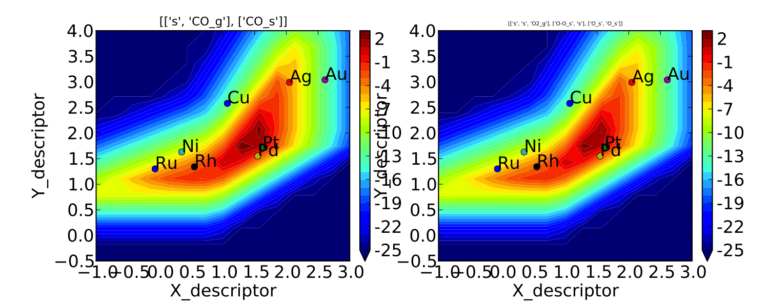
This looks pretty similar to previously published results by Falsig et. al., with minor differences to be expected since the model and inputs used here are slightly different.
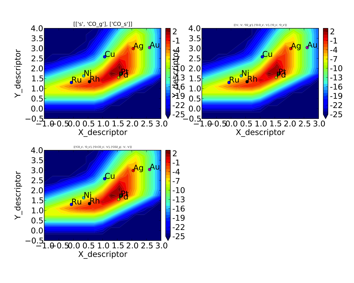
We notice that the rates are given for CO adsorption and oxygen adsorption, but that associative CO2 desorption is not included. This is because it is identical to the plot for CO adsorption (due to the steady-state condition). If we want to include it we can do:
vm.unique_only = False
vm.plot('all_rates.pdf')
vm.unique_only = True
(we turn it back to unique_only right afterwards since this is
generally less cluttered)
which gives us a plot for each elementary step:
We might also be interested in the production rate of CO2 rather than
the rates of elementary steps (it is trivial to see that they are
equivalent here, but this is not always the case). If we want to analyze
this we need to include the “production_rate” in the outputs, re-run
the model, and re-plot.
model.output_variables += ['production_rate']
model.run()
vm.production_rate_map = model.production_rate_map #attach map
vm.threshold = 1e-30 #do not plot rates below this
vm.plot_variable = 'production_rate'
vm.plot(save='production_rate.pdf')
In the line commented “attach map” we point the VectorMap instance to the new output from the model. This line is not necessary if the output had been included in the original “output_variables”. We also note that the “threshold” variable will be discussed in the next tutorial.
Now we can see whats going on, but its not very pretty (the colorbar is cutoff). We can make a few aesthetic improvements fairly simply:
vm.descriptor_labels = ['CO reactivity [eV]', 'O reactivity [eV]']
vm.subplots_adjust_kwargs = {'left':0.2,'right':0.8,'bottom':0.15}
vm.plot(save='pretty_production_rate.pdf')
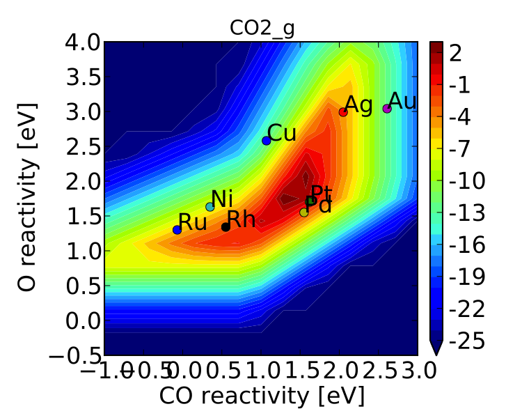
Ok, so its still not publishable, but its better. There are ways to control the finer details of the plots, but that will come in a later tutorial.
One more thing we might be interested in is the coverages of various intermediates. This can also be plotted with the VectorMap (since coverages are output as a 1-dimensional “vector”). However, we are going to want to make a few changes to the settings:
vm.plot_variable = 'coverage'
vm.log_scale = False
vm.min = 0
vm.max = 1
vm.plot(save='coverage.pdf')
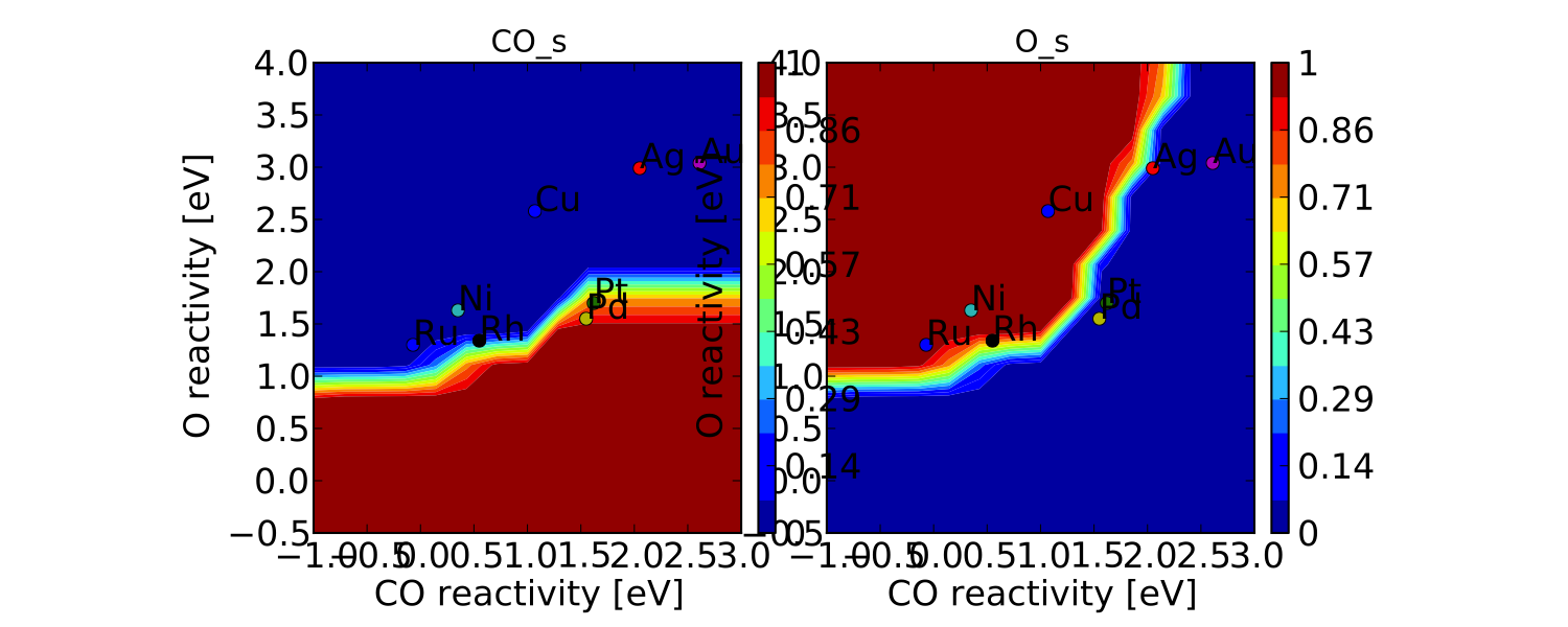
Not the prettiest plot ever, but you get the point. We could re-adjust the subplots_adjust_kwargs to make this more readable, but that is left as an independent exercise.
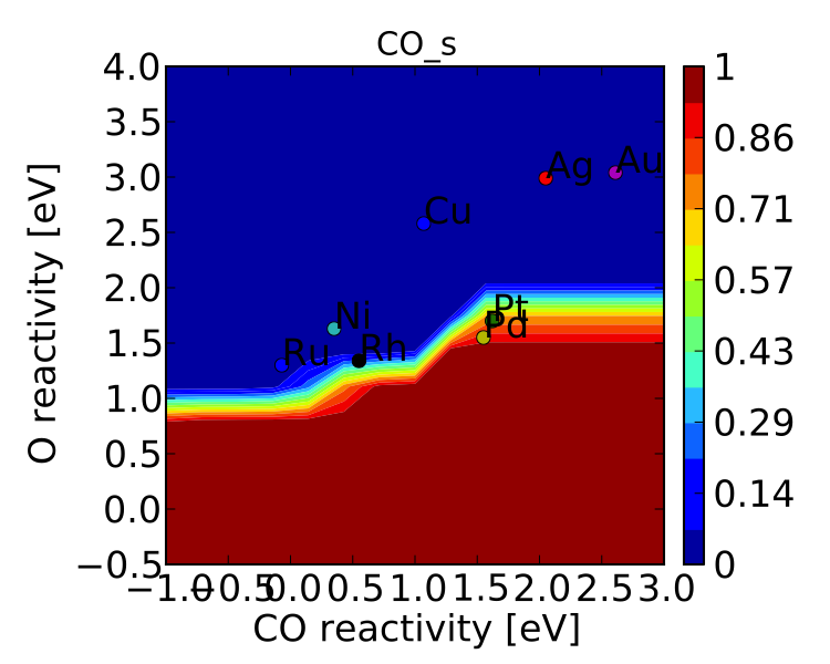
Finally, we might not always be interested in seeing all of the coverages. If we only wanted to see the CO coverage we could specify this by:
vm.include_labels = ['CO_s']
vm.plot(save='CO_coverage.pdf')
Note that the strings to use in “include_labels” can be found by
examining the “output_labels” dictionary from the log
file; alternatively you can specify
“include_indices = [0,1,...]” where the integers correspond to the
indices of the plots to include.