Including Adsorbate-Adsorbate Interactions

Warning

The support of adsorbate-adsorbate interactions in CatMAP is currently undergoing significant changes. This will produce backwards-incompatible changes and this tutorial will change accordingly.

In all of the previous tutorials we have made some assumptions about how the adsorbed species interact with the surface lattice and each other. Specifically, we assume that every species adsorbs at a single site and does not interact with its neighbors. In this tutorial we will examine these assumptions more closely and consider some strategies for making more advanced assumptions. Please note that while most of the other features of CatMAP are relatively well tested, the features outlined in this tutorial have had very little testing/error checking so please be careful if using them in your research (and naturally let the developers list know about any issues).

It is also worth mentioning that while “ideal” mean-field models like the ones shown previously are usually mathematically well-behaved and thus exhibit “existence and uniqueness” (there is one and only one steady-state solution), all bets are off once adsorbate interactions are included. Thus it is likely possible to construct models which have oscillating solutions or no solutions at all (within the physical bounds). Naturally a system with no solution at all is unphysical, so as long as you make good assumptions then you should be okay. However, oscillating solutions are slightly trickier and it can be very hard to determine if/when this is an issue since CatMAP uses root finding to get the steady-state solution. I have yet to come across an example where CatMAP cannot find a solution to a realistic model, but be aware that it could happen.

We will continue with the CO oxidation example to avoid having to create completely new files. The tutorials will seek to demonstrate the options available within CatMAP, even if these options are not physical for the CO oxidation system, so don’t take the outputs too seriously. The tutorial is divided into 2 parts which do not necessarily need to be followed sequentially:

• Multi-site adsorbates and maximum coverages
• Coverage dependent adsorption energies

For both sections we will use a submission script (mkm_job.py) similar to the one in the Using Thermodynamic Descriptors tutorial:

from catmap import ReactionModel

mkm_file = 'CO_oxidation.mkm'
model = ReactionModel(setup_file=mkm_file)
model.output_variables += ['production_rate']
model.run()

from catmap import analyze
vm = analyze.VectorMap(model)
vm.plot_variable = 'production_rate' #tell the model which output to plot
vm.log_scale = True #rates should be plotted on a log-scale
vm.min = 1e-25 #minimum rate to plot
vm.max = 1e8 #maximum rate to plot
vm.threshold = 1e-25 #anything below this is considered to be 0
vm.subplots_adjust_kwargs = {'left':0.2,'right':0.8,'bottom':0.15}
vm.plot(save='production_rate.pdf')

vm.plot_variable = 'coverage' #tell the model which output to plot
vm.log_scale = False #coverage should not be plotted on a log-scale
vm.min = 0 #minimum coverage
vm.max = 1 #maximum coverage
vm.subplots_adjust_kwargs = {'left':0.2,'right':0.8,'bottom':0.15,'wspace':0.6}
vm.plot(save='coverage.pdf')

We use the same input file (energies.txt) and start with the same setup file (CO_oxidation.mkm) from Tutorial 2 . Note that each section assumes you are starting with the “fresh” CO_oxidation.mkm file from Tutorial 2.

Multi-site adsorbates and maximum coverages

One very simple way of including adsorbate interactions is the “hard sphere exclusion” model. Actually, we have already assumed this (each site can have only 0 or 1 adsorbate), but we can also extend the assumption to allow adsorbates to occupy more than 1 site, or to set a “maximum coverage” for an adsorbate. Lets take a look at the multi-site adsorbates first:

Multi-site adsorption

CatMAP includes the ability to allow and adsorbate to adsorb to multiple sites of the same type. For instance, lets say that we want to force CO to adsorb to 2 sites. This is achieved by editing the “rxn_expressions”:

rxn_expressions = [

               '2*_s + CO_g -> CO*',
               '2*_s + O2_g <-> O-O* + *_s -> 2O*',
               'CO* +  O* <-> O-CO* + 2* -> CO2_g + 3*',

                   ]

Note that we had to edit the number of sites on the CO adsorption and desorption reactions in order to make everything consistent. The next thing we need to do is tell CatMAP that CO occupies 2 sites, so that it doesn’t get confused about the site balance:

species_definitions['CO_s'] = {'n_sites':2}

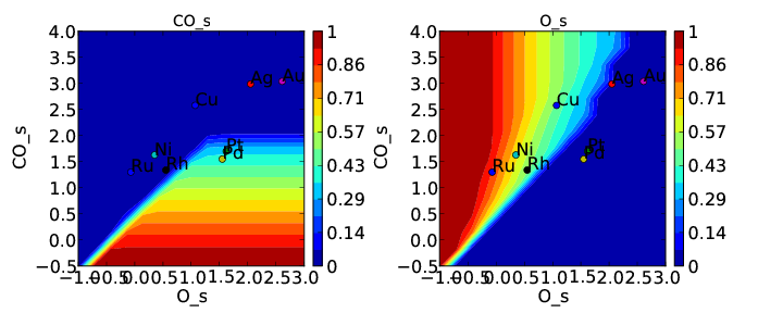
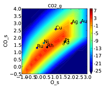
Now we can run the model and get the following coverages:

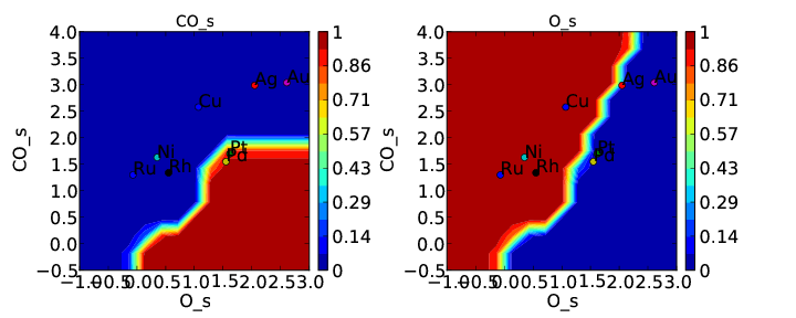
and rate:

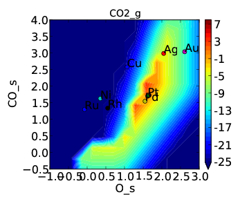
If we compare these to Tutorial 2 then we can see that the CO* coverage is suppressed and there is more O* in the bottom left of the plot. This is what we would expect to happen when we require an adsorbate to have an extra free site to adsorb.

There is one thing worth noting about this approach. If coverage was defined as number of CO per number of surface sites we would expect the maximum CO coverage to be 0.5 since it occupies 2 sites. However, it is clear from the plot that the coverage goes to 1. That is because we have re-defined the number of “total sites” to be a factor of 2 less for CO so that the maximum coverage of an adsorbate is always 1. This is equivalent to assuming that the probability of an adsorbate which occupies 2 sites reacting with another adsorbate is a factor of 2 higher since the site it sits on is 2 times larger. Depending on the system this may be a poor assumption, but it is the only option currently implemented in CatMAP.

Maximum coverages

There may also be circumstances where we wish to constrain certain adsorbates to have a maximum coverage. This can easily be achieved by adding the line:

species_definitions['CO_s'] = {'max_coverage':0.5}

to CO_oxidation.mkm. However, when you run the submission script you will notice that after a lot of complaining CatMAP will give the following:

mapper_iteration_3: fail - no solution at 99 points.

This is the first time we have encountered a model that will not converge. Normally we would try to get convergence by increasing “max_bisections” or other parameters as discussed in Tutorial 3. However, in this case it is hopeless. This is probably because there is no solution within the bounds we have defined (which means they are not physical). This isn’t too surprising since we just made the constraint up. We can still take a look at the points that did converge in coverages.pdf:

This is pretty consistent with what we might expect. The model converges everywhere that CO coverage is less than 0.5 in the unconstrained solution, but starts to break down when the constraint limits the CO coverage to less than what is found in the unconstrained solution. Although this approach does not really make physical sense here, there could be systems where it does. In these cases CatMAP should be able to find a valid solution. Note that the “max_coverage” only pertains to one adsorbate, and does not inhibit competitive adsorption (i.e. you could have CO coverage of 0.5 and O coverage of 0.5).

Coverage dependent adsorption eneriges

A more powerful method for including adsorbate-adsorbate interactions is to allow adsorption energies to depend on the coverages the adsorbates. This is still relatively crude compared to an explicit lattice method like kinetic Monte Carlo, but it should provide a good picture of the first-order effects of coverage . Of course there are many ways to parameterize such a model, but there is currently only one option implemented in CatMAP - the “first order adsorption energy” model. We will first introduce the model, then look at how to use it in CatMAP, and finally show an example of how to apply it to the CO oxidation example.

First order adsorption energy model

In this model we assume that adsorption energies follow the following relationship:

\[\begin{split}E_{i} =& E_{i}^{i} + \sum_{j} {\cal{F} (|\theta|_{j}) \varepsilon_{ij} \theta_{j}} \\ |\theta|_j =& \sum_{{\mathrm{site}_k}={\mathrm{site}_j}} \theta_{k}\end{split}\]

where \(E_{i}\) is the generalized formation energy for species \(i\), |θ|j is the total coverage of occupied sites for the site on which adsorbate \(j\) is adsorbed, \(\varepsilon_{ij}\) is the “interaction matrix”, and F is the “interaction response function” which is usually some smoothed piecewise linear function and will be discussed later. When computing the Jacobian matrix for the system we will also need the derivative of the energy with respect to coverages. This is given by:

\[\frac{\partial E_{i}}{\partial \theta_l} = \sum_{j} \varepsilon_{ij} \left( \frac{\rm{d} \cal{F} \left(|\theta|_j\right)}{\rm{d}|\theta|_j} \frac{\rm{d}|\theta|_j}{\rm{d}\theta_{l}} \theta_{j} + \cal{F} \left(|\theta|_j\right)\delta_{jl} \right)\]

The model is called “first order” since it includes only one term of coverage dependence, and this term is first order in the coverage (and \(\cal{F}\)).

We see that in order to calculate adsorption energies we need the function \(\cal{F}\), and the matrix \(\varepsilon\). We will also end up needing the derivative of the function \(\cal{F}\) w.r.t. \(|θ|_j\) . These two quantities will be discussed below.

Interaction response function

The “interaction response function” determines how much the adsorption energy changes as a function of the total coverage at a site. This is necessary because adsorption energies often follow non-linear behavior as a function of coverage. Some examples of possible response functions are shown below:

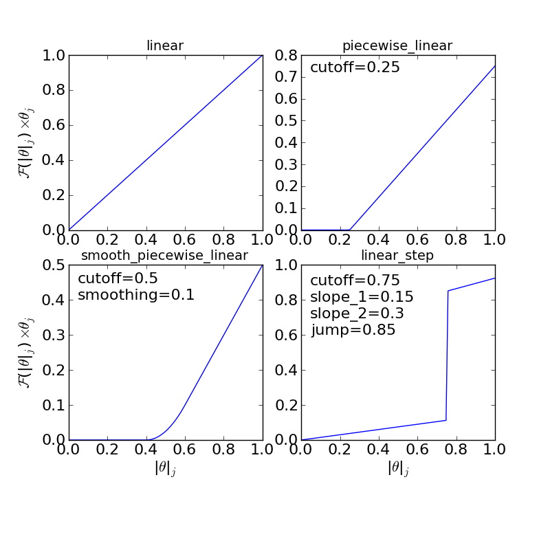
The “linear”, “piecewise_linear”, and “smooth_piecewise_linear” are implemented in CatMAP, while the “linear_step” is a hypothetical model which could be implemented. Depending on the complexity of the interaction response function it will require some parameters. The parameters are “site specific”, so that if you have a model with step sites and terrace sites you could use different “cutoffs” for the piecewise linear response function. However, the parameters do not vary by adsorbate which limits the complexity of the model.

Interaction matrix

The other key input for the “first order” interaction model is the “interaction matrix”, εij. There are two types of terms in this matrix - “self interaction” terms (\(\varepsilon_{ii}\)) and “cross interaction” terms (\(\varepsilon_{ij} (i\ne j)\)). As the name suggests the “self interaction” terms tell how much an adsorbate interacts with itself, while “cross interactions” tell how much it interacts with other adsorbates. The interaction matrix is symmetric (\(\varepsilon_{ij} = \varepsilon_{ji}\)). The values for the matrix are determined by fitting to data. If the differential binding energies are available at various coverages then the fitting is very straight-forward. However, in most cases density functional theory (DFT) will be used to calculate binding energies. Due to the discreet nature of coverages in DFT, it is impossible to calculate differential binding energies. Instead, average binding energies are calculated and used to obtain the interaction parameters. The definition of average binding energy is:

\[\begin{split}\bar{E}_i =& \frac{\int_{0}^{\theta_i} E_{i} \rm{d} \theta_{i}}{|\theta|_i} \\ =& \frac{\int_0^{\theta_i} \left(E_i^0 + \sum_k \cal{F}(|\theta|_k)\varepsilon_{ik}\theta_k \right) \rm{d}\theta_i}{|\theta|_i}\end{split}\]

from this we can solve for the self-interaction parameters:

These equations look nasty at first site, but the form of \(\cal{F}\) is usually simple enough that they aren’t so intimidating. CatMAP also includes the ability to fit the self-interaction functions automatically, as discussed later.

The cross interaction terms are very costly to calculate, since they require many DFT calculations (two per adsorbate per adsorbate, or Nadsorbates2). For this reason it is common to use some approximations. The most common approximations are:

\[\begin{split}{\mathrm{geometric\ mean:}}\ \varepsilon_{ij} =& \sqrt{|\varepsilon_{ii} \varepsilon_{jj}|} \\ {\mathrm{arithmetic\ mean:}}\ \varepsilon_{ij} =& (\varepsilon_{ii} + \varepsilon_{j})/2\\ {\mathrm{ neglect:}}\ \varepsilon_{ij} =& 0\end{split}\]

In CatMAP the cross interaction terms are between adsorbate-adsorbate and adsorbate-transition_states. This means that the interaction matrix is actually (Nadsorbate+Ntransition-state)2. Both self and cross interactions between transition states are neglected since by definition their coverage will always be negligible. However, cross interactions between adsorbates and transition-states is not negligible. Since we don’t have any self-interaction parameters for transition-states, we need some method of estimating them. This can be done by:

• transition-state scaling: transition-state scaling is used to estimate the cross parameters so that the transition-state scaling relation holds (best approximation if available)
• initial state: use the cross interaction parameters corresponding to the initial state (forward barrier is static)
• final state: use the cross interaction parameters corresponding to the final state (reverse barrier is static)
• intermediate state: use some weighted average of the initial and final state interactions (usually 0.5).
• neglect: assume to be 0 (all barriers decrease)

Implementation in CatMAP

The implementation of adsorbate-interactions requires modifications at many levels of CatMAP - specifically, the solver, scaler, and parser have been modified for the first order interaction model. However, the place that the “interactions” fit most logically into the design of CatMAP is in the “thermodynamics” since technically this is a modification of the assumption of non-interacting adsorbates. For this reason, most of the implementation has been abstracted into a class which is in the thermodynamics directory. If you are not developing then this is not a concern, but just be aware that in order to use the “first order” interaction model (or others in the future) you need to ensure that the parser, scaler, and solver are compatible. Currently the default parser (TableParser), scaler (GeneralizedLinearScaler), and solver (SteadyStateSolver) are the only ones compatible with interaction models.

Relevant Attributes

The implementation relies on the following attributes of the reaction model:

• adsorbate_interaction_model: Determines which model to use. Currently can be ‘ideal’ (default) or ‘first_order’

• interaction_response_function: The function \(F\) from above. Can be ‘linear’, ‘piecewise_linear’, or ‘smooth_piecewise_linear’. Can also be a callable function which takes the total coverage of a site as its first argument and the “interaction_response_parameters” dictionary as a **kwargs argument. Must return the value and derivative of the function at the specified total coverage.

• interaction_response_parameters: This is a dictionary of argument names/values to be used in the “interaction_response_function”. The “interaction_response_parameters” can be specified as an attribute of the ReactionModel (use the same parameters for all sites) or as a key/value in the “species_definitions” dictionary for different sites (use different parameters for different sites).

• self_interaction_parameters: These are the self interaction parameters for a given adsorbate. They should be specified as a key/value in the species definition entry for the adsorbate. The key should be “self_interaction_parameters” and the value should be a list of the same length as “surface_names”. The parameters should be entered for each surface in the same order that the surfaces appear in “surface_names”. If an interaction parameter is not available for a surface then None should be entered.

• cross_interaction_parameters: Cross-interaction parameters can be input as a key/value pair in the species_definitions entry for one of the two adsorbates. The key should be “cross_interaction_parameters” and the value should be a dictionary where the key is the other adsorbate of the cross interaction pair and the value is a list of the same length as “surface names” where the parameters are input similar to the “self_interaction_parameters”. The following is an example of how this might appear in the setup file for neglecting CO-O cross interactions on Pt, Pd, and Rh:

  ...
  surface_names = ['Pt','Pd','Rh']
  ...
  species_definitions['CO_s'] = {'cross_interaction_parameters':{'O_s':[0,0,0]}}
  ..
  

  Explicitly specifying cross interaction parameters is optional. Any parameters that are not explicitly specified will be estimated as specified by “cross_interaction_mode”. Note that one parameter must be specified for each surface, and None can be used if a value is unknown. The “surface_names” in the example above is the same “surface_names” which defines the surfaces in the entire model, and thus should only be defined once.

• max_self_interaction: Practically it is sometimes found that the self interaction parameter should not be larger than some cutoff. This can be specified by setting the “max_self_interaction” key in the species_definitions dictionary for the adsorbate to either the numerical value or a name of one of the “surface_names” to automatically bound the interaction parameter at the value for that surface. The attribute can also be added directly to the ReactionModel in order to bound all self interaction parameters (for this, especially, using a “surface name” as a bound is recommended).

• cross_interaction_mode: The cross interaction mode tells CatMAP how to approximate cross interaction parameters that are not specified explicitly. The values can be: ‘geometric_mean’ (default), ‘arithmetic_mean’ or ‘neglect’ as described above.

• transition_state_cross_interaction_mode: Similar to “cross_interaction_mode” but for transition-states. Can be ‘transition_state_scaling’, ‘initial_state’, ‘final_state’, ‘intermediate_state’, or ‘neglect’ as described above. Using ‘intermediate_state’ will assume a weight of 0.5, or you can specify ‘intermediate_state(X)’ to set a weight of X.

• interaction_scaling_constraint_dict: The equivalent of “scaling_constraint_dict” but for interaction parameters. By default, “scaling_constraint_dict” will be used, but constraints which force slopes to be positive/negative will be removed since sign changes are expected between the “adsorbate scaling” coefficient and the interaction parameter scaling coefficient. Any parameter which does not have scaling constraints defined will be set to the “default_interaction_constraints” attribute ([None,None,None] by default).. Cross interaction parameter names are defined by ‘A&B’ and can appear in either order. For example, to constrain the cross parameter between O* and CO* to scale only with the first descriptor we could do:

  interaction_scaling_constraint_dict['O_s&CO_s'] = [None,0,None]
  

  Defining the constraint for ‘CO_s&O_s’ would be equivalent. See Tutorial 2 for a refresher on the syntax of constraint definitions.

• non_interacting_site_pairs: Pairs of site names which are not interacting. All cross interactions between adsorbates on these sites will be set to 0. For example, to prevent cross interactions between adsorbates on the ‘s’ and ‘t’ site:

  non_interacting_site_pairs = [['s','t']]
  

  The order of adsorbates does not matter since the interaction matrix is symmetric.

• interaction_strength: All interaction parameters will be multiplied by this. Should be floatable. Defaults to 1. Useful for getting model to converge.

• interaction_fitting_mode: Determines how to construct fits to raw data. Can be None (default), ‘average_self’. None implies that CatMAP should not try to automatically do any fitting because the parameters are explicitly specified. Using “average_self” will fit the self interaction parameters assuming that there are coverage-dependent average adsorption energies in the input file.

In addition, the interaction matrix can be included as an output for error-checking (this is recommended since the interaction model is still relatively new). Simply include “interaction_matrix” in the “output_variables” and analyze the output as described in Tutorial 2 <../tutorials/creating_a_microkinetic_model>.

CO Oxidation Example

Including coverage-dependent interactions

First, lets assume that we already know the self-interaction parameters and want to include coverage dependent adsorbate interactions on top of the model discussed in Tutorial 2. In order to do this we need to add the following to the CO_oxidation.mkm setup file:

adsorbate_interaction_model = 'first_order' #use "first order" interaction model
interaction_response_function = 'smooth_piecewise_linear' #use "smooth piecewise linear" interactions
species_definitions['s']['interaction_response_parameters'] = {'cutoff':0.25,'smoothing':0.01}
#input the interaction paramters
#surface_names = ['Pt', 'Ag', 'Cu','Rh','Pd','Au','Ru','Ni'] #surface order reminder
species_definitions['CO_s'] = {'self_interaction_parameter':[3.248, 0.965, 3.289, 3.209, 3.68, None, None, None]}
species_definitions['O_s'] = {'self_interaction_parameter':[3.405, 5.252, 6.396, 2.708, 3.87, None, None, None]}
max_self_interaction = 'Pd' #self interaction parameters cannot be higher than the parameter for Pd
transition_state_cross_interaction_mode = 'transition_state_scaling' #use TS scaling for TS interaction
cross_interaction_mode = 'geometric_mean' #use geometric mean for cross parameters

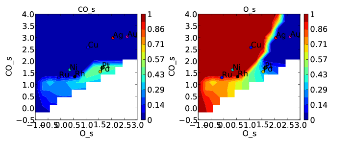
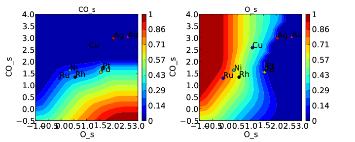
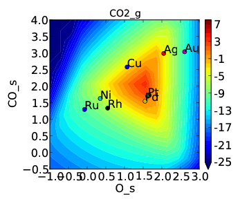
If we use the same submission script as before we should get the following outputs for coverage and rate:

We can see that the coverages change much more gradually, as expected. The rate volcano is a little worrying since it now predicts Pt and Pd to be some of the worst catalysts. However, we recall that the reaction mechanism here is very simplistic, and that we are only looking at the (111) surfaces. A more realistic analysis would reveal that Pt and Pd are still the optimal catalysts, as shown by Grabow et. al..

Including scaled cross interactions

In the previous section we used the “geometric mean” approximation to get the cross-interaction terms from the self-interaction terms. While this is a good first approximation, it is sometimes not sufficiently accurate. In order to account for this it is possible to also include some cross-interaction terms as scaled parameters. For a very unphysical example, we will neglect cross-interactions between adsorbed O and CO, and between adsorbed CO and the O-O transition-state. This can be done by adding the following to the species definition for adsorbed CO:

species_definitions['CO_s'] = {'self_interaction_parameter':[3.248, 0.965, 3.289, 3.209, 3.68, None, None, None],
                    'cross_interaction_parameters':{'O_s':[0,0,0,0,0,0,0,0],'O-O_s':[0,0,0,0,0,0,0,0]}}

We note that the cross interactions could have equivalently been defined in the species definitions for adsorbed O and the O-O transition-states (where CO_s would be the key of the cross_interaction_parameters dictionary) but it is easier to group them both into the CO_s definition. If we now run the submission script we get the following outputs:

These results are not physical because there is no reason to expect that CO does not interact with O or O-O, but they do illustrate the syntax for specifying arbitrary cross interaction parameters. Note that the vector of zeroes here is the same length as the number of surfaces. Much like the self interaction parameters, the values of these cross interactions must be in the same order as the order of the surface names, with any unknown parameters given as None. If actual parameters were input instead of zeroes, then they would also be estimated using scaling relations in the same way the self interaction parameters are.

Using CatMAP to fit self interactions

In many cases the interaction parameters will not be available and they must be determined from some set of coverage dependent raw data. In this situation it is very convenient to have the interaction matrix automatically fit to this raw data to avoid typos and round off error in the interaction parameters. CatMAP is capable of automatically constructing this fit for the self-interaction parameters of the “first order” model described above. Fitting the second order parameters is more complicated, and should be done manually. In order to create the automatic fit it is necessary to have the energies as a function of coverage. For example, we can use the following input file with some soon to be published data for coverage dependent O and CO adsorption, along with transition-state energies from previous examples. Note that there is now a new “coverage” column:

surface_name    site_name   species_name    coverage    formation_energy    bulk_structure  frequencies other_parameters    reference
None    gas CO2 0   2.46    None    [1333,2349,667,667] []  "NIST"
None    gas CO  0   2.77    None    [2170]  []  "Energy Environ. Sci., 3, 1311-1315 (2010)"^M
None    gas O2  0   5.42    None    [1580]  []  NIST^M
Rh  111 O   0.25    0.54    fcc []  []  Khan et. al. Parameterization of an interaction model for adsorbate-adsorbate interactions
Pt  111 O   0.25    1.62    fcc []  []  Khan et. al. Parameterization of an interaction model for adsorbate-adsorbate interactions
Pd  111 O   0.25    1.55    fcc []  []  Khan et. al. Parameterization of an interaction model for adsorbate-adsorbate interactions
Cu  111 O   0.25    1.08    fcc []  []  Khan et. al. Parameterization of an interaction model for adsorbate-adsorbate interactions
Ag  111 O   0.25    2.04    fcc []  []  Khan et. al. Parameterization of an interaction model for adsorbate-adsorbate interactions
Au  111 O   0.25    2.75    fcc []  []  Khan et. al. Parameterization of an interaction model for adsorbate-adsorbate interactions
Rh  111 O   0.50    0.76    fcc []  []  Khan et. al. Parameterization of an interaction model for adsorbate-adsorbate interactions
Pt  111 O   0.50    1.9 fcc []  []  Khan et. al. Parameterization of an interaction model for adsorbate-adsorbate interactions
Pd  111 O   0.50    1.88    fcc []  []  Khan et. al. Parameterization of an interaction model for adsorbate-adsorbate interactions
Cu  111 O   0.50    1.755   fcc []  []  Khan et. al. Parameterization of an interaction model for adsorbate-adsorbate interactions
Ag  111 O   0.50    2.585   fcc []  []  Khan et. al. Parameterization of an interaction model for adsorbate-adsorbate interactions
Au  111 O   0.50    3.065   fcc []  []  Khan et. al. Parameterization of an interaction model for adsorbate-adsorbate interactions
Rh  111 O   0.75    1.043   fcc []  []  Khan et. al. Parameterization of an interaction model for adsorbate-adsorbate interactions
Pt  111 O   0.75    2.243   fcc []  []  Khan et. al. Parameterization of an interaction model for adsorbate-adsorbate interactions
Pd  111 O   0.75    2.237   fcc []  []  Khan et. al. Parameterization of an interaction model for adsorbate-adsorbate interactions
Cu  111 O   0.75    2.423   fcc []  []  Khan et. al. Parameterization of an interaction model for adsorbate-adsorbate interactions
Ag  111 O   0.75    3.147   fcc []  []  Khan et. al. Parameterization of an interaction model for adsorbate-adsorbate interactions
Au  111 O   0.75    3.5 fcc []  []  Khan et. al. Parameterization of an interaction model for adsorbate-adsorbate interactions
Rh  111 O   1.00    1.31    fcc []  []  Khan et. al. Parameterization of an interaction model for adsorbate-adsorbate interactions
Pt  111 O   1.00    2.592   fcc []  []  Khan et. al. Parameterization of an interaction model for adsorbate-adsorbate interactions
Pd  111 O   1.00    2.665   fcc []  []  Khan et. al. Parameterization of an interaction model for adsorbate-adsorbate interactions
Cu  111 O   1.00    2.925   fcc []  []  Khan et. al. Parameterization of an interaction model for adsorbate-adsorbate interactions
Ag  111 O   1.00    3.55    fcc []  []  Khan et. al. Parameterization of an interaction model for adsorbate-adsorbate interactions
Au  111 O   1.00    3.797   fcc []  []  Khan et. al. Parameterization of an interaction model for adsorbate-adsorbate interactions
Rh  111 CO  0.25    1.25    fcc []  []  Khan et. al. Parameterization of an interaction model for adsorbate-adsorbate interactions
Pt  111 CO  0.25    1.49    fcc []  []  Khan et. al. Parameterization of an interaction model for adsorbate-adsorbate interactions
Pd  111 CO  0.25    1.3 fcc []  []  Khan et. al. Parameterization of an interaction model for adsorbate-adsorbate interactions
Cu  111 CO  0.25    2.53    fcc []  []  Khan et. al. Parameterization of an interaction model for adsorbate-adsorbate interactions
Ag  111 CO  0.25    2.96    fcc []  []  Khan et. al. Parameterization of an interaction model for adsorbate-adsorbate interactions
Rh  111 CO  0.50    1.58    fcc []  []  Khan et. al. Parameterization of an interaction model for adsorbate-adsorbate interactions
Pt  111 CO  0.50    1.915   fcc []  []  Khan et. al. Parameterization of an interaction model for adsorbate-adsorbate interactions
Ag  111 CO  0.50    3.07    fcc []  []  Khan et. al. Parameterization of an interaction model for adsorbate-adsorbate interactions
Rh  111 CO  1.00    2.193   fcc []  []  Khan et. al. Parameterization of an interaction model for adsorbate-adsorbate interactions
Pt  111 CO  1.00    2.473   fcc []  []  Khan et. al. Parameterization of an interaction model for adsorbate-adsorbate interactions
Pd  111 CO  1.00    2.335   fcc []  []  Khan et. al. Parameterization of an interaction model for adsorbate-adsorbate interactions
Cu  111 CO  1.00    3.455   fcc []  []  Khan et. al. Parameterization of an interaction model for adsorbate-adsorbate interactions
Ag  111 CO  1.00    3.247   fcc []  []  Khan et. al. Parameterization of an interaction model for adsorbate-adsorbate interactions
Rh  111 O-CO    0.25    3.1 fcc []  []  "Angew. Chem. Int. Ed., 47, 4835 (2008)"
Pt  111 O-CO    0.25    4.04    fcc []  []  "Angew. Chem. Int. Ed., 47, 4835 (2008)"
Pd  111 O-CO    0.25    4.2 fcc []  []  "Angew. Chem. Int. Ed., 47, 4835 (2008)"
Cu  111 O-CO    0.25    4.18    fcc []  []  "Angew. Chem. Int. Ed., 47, 4835 (2008)"
Ag  111 O-CO    0.25    5.05    fcc []  []  "Angew. Chem. Int. Ed., 47, 4835 (2008)"
Au  111 O-CO    0.25    5.74    fcc []  []  "Angew. Chem. Int. Ed., 47, 4835 (2008)"
Rh  111 O-O 0.25    3.79    fcc []  []  Falsig et al (2012)
Pt  111 O-O 0.25    5.35    fcc []  []  Falsig et al (2012)
Pd  111 O-O 0.25    5.34    fcc []  []  Falsig et al (2012)
Cu  111 O-O 0.25    4.74    fcc []  []  Falsig et al (2012)
Ag  111 O-O 0.25    5.98    fcc []  []  Falsig et al (2012)
Au  111 O-O 0.25    7.22    fcc []  []  Falsig et al (2012)

Naturally the transition-states only need to be computed at a single coverage, since they do not have self interaction parameters. It is also worth noting that even if not all metals have coverage dependent data, they can still be included in the analysis (their interaction parameters will be estimated from scaling).

You can find the above data table as coverage_energies.txt in the folder for this tutorial. If you make the following changes to CO_oxidation.mkm then the parameters will be determined automatically:

input_file = 'coverage_energies.txt'
interaction_fitting_mode = 'average_self'

The “average_self” fitting mode refers to the fact that the energies in the input file are average adsorption energies, and that only the self interaction parameters will be fit. The only other option is “differential_self” which assumes that the inputs are differential adsorption energies and fits self interaction parameters.

Now, if you run mkm_job.py then you will get the same output as when the self interaction parameters were input manually (because the parameters were pre-determined by this procedure). If you want to view the parameters then you can do so by looking at the “self_interaction_parameter_dict” in the CO_oxidation.log. You should notice that they match the parameters that were input manually earlier. The advantage of the automatic fitting procedure is that any changes in the “interaction response function” will automatically be compensated for in the fit (i.e. if the smoothing value is decreased, cutoff is changed, etc.). It also makes it easier to generalize the model to inputs coming from different calculation methods, functionals, etc.