Refining a Microkinetic Model¶

In this tutorial we will take the simple CO oxidation model presented in Creating a Microkinetic Model and refine it to be more complete. This tutorial should show some of the more powerful capabilities of CatMAP, and highlight the ability to dynamically make changes to the kinetic model with minimal programming. The tutorial will show several possibilities of ways to refine the model towards something that correctly represents the physical system:

Adding elementary steps (refining the mechanism)
Adding multiple sites (refining the active site structure)
Sensitivity analyses (refining the inputs to the model)
Refining numerical accuracy (resolution, tolerance, etc.)

These sections do not need to be followed sequentially. For each one we will start with the same setup file and input file from Creating a Microkinetic Model. We will use a slightly more efficient submission script:

from catmap import ReactionModel

mkm_file = 'CO_oxidation.mkm'
model = ReactionModel(setup_file=mkm_file)
model.output_variables += ['production_rate']
model.run()

from catmap import analyze
vm = analyze.VectorMap(model)
vm.plot_variable = 'production_rate' #tell the model which output to plot
vm.log_scale = True #rates should be plotted on a log-scale
vm.min = 1e-25 #minimum rate to plot
vm.max = 1e3 #maximum rate to plot

vm.descriptor_labels = ['CO reactivity [eV]', 'O reactivity [eV]']
vm.threshold = 1e-25 #anything below this is considered to be 0
vm.subplots_adjust_kwargs = {'left':0.2,'right':0.8,'bottom':0.15}
vm.plot(save='pretty_production_rate.pdf')

Adding Elementary Steps¶

One way of refining a model is to include additional steps in the mechanism. To demonstrate this we will add molecular adsorption of oxygen prior to dissociation. In order to do this we need to include the relevant energetics, so add the following lines to the energies.txt:

Ru  111 O2  3.15    fcc []  []  "Angew. Chem. Int. Ed., 47, 4835 (2008)"
Rh  111 O2  3.63    fcc []  []  "Angew. Chem. Int. Ed., 47, 4835 (2008)"
Ni  111 O2  3.76    fcc []  []  "Angew. Chem. Int. Ed., 47, 4835 (2008)"
Pd  111 O2  4.29    fcc []  []  "Angew. Chem. Int. Ed., 47, 4835 (2008)"
Cu  111 O2  4.52    fcc []  []  "Angew. Chem. Int. Ed., 47, 4835 (2008)"
Pt  111 O2  4.56    fcc []  []  "Angew. Chem. Int. Ed., 47, 4835 (2008)"
Ag  111 O2  5.1 fcc []  []  "Angew. Chem. Int. Ed., 47, 4835 (2008)"

Next, we just need to define the new elementary step in the setup file (CO_oxidation.mkm):

rxn_expressions = [

                '*_s + CO_g -> CO*',
#               '2*_s + O2_g <-> O-O* + *_s -> 2O*',
                '*_s + O2_g -> O2_s',
                '*_s + O2_s <-> O-O* + *_s -> 2O*',
                'CO* +  O* <-> O-CO* + * -> CO2_g + 2*',

                    ]

Now we can run mkm_job.py to get the output. If you run in a clean directory you should see something like:

mapper_iteration_0: status - 225 points do not have valid solution.
minresid_iteration_0: success - [ 3.00, 4.00] using coverages from [ 3.00, 4.00]
minresid_iteration_0: success - [ 3.00, 3.68] using coverages from [ 3.00, 3.68]
minresid_iteration_0: success - [ 3.00, 3.36] using coverages from [ 3.00, 3.36]
minresid_iteration_0: success - [ 3.00, 3.04] using coverages from [ 3.00, 3.04]
minresid_iteration_0: success - [ 3.00, 2.71] using coverages from [ 3.00, 2.71]
...
minresid_iteration_1: success - [-1.00, 0.14] using coverages from [-1.00, 0.46]
rootfinding_iteration_2: fail - stagnated or diverging (residual = 3.85907297979e-29)
minresid_iteration_0: fail - [-1.00,-0.18] using coverages from [-1.00,-0.18]; initial residual was 8.73508143601e-21 (residual = 3.85907297979e-29)
minresid_iteration_1: success - [-1.00,-0.18] using coverages from [-1.00, 0.14]
minresid_iteration_0: success - [-1.00,-0.50] using coverages from [-1.00,-0.50]
mapper_iteration_1: status - 0 points do not have valid solution.

However, if you run in the same directory that you used for Creating a Microkinetic Model, you will see slightly different output. Either way, the model should converge.

If you look at “pretty_production_rate.pdf” it should look like the following:

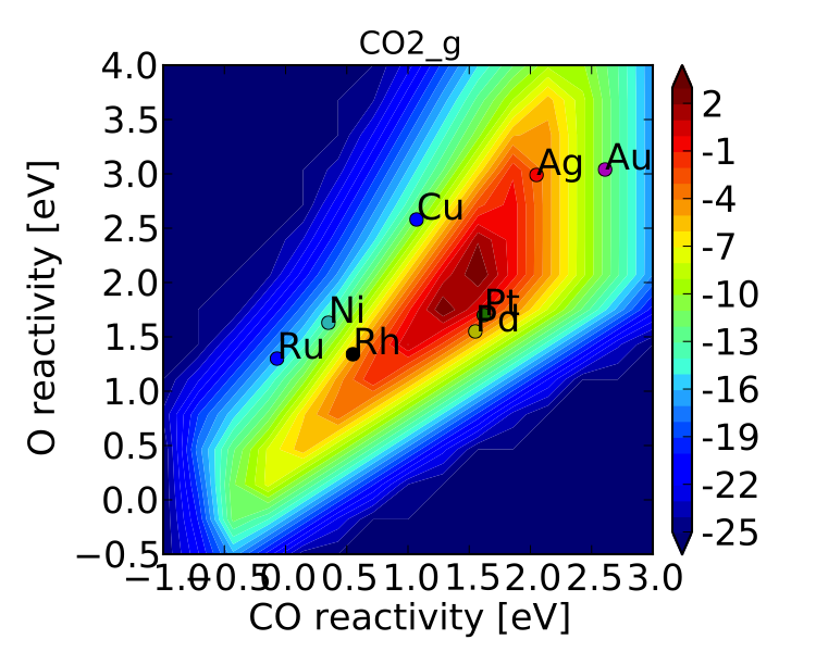
If we compare this to the figure from the previous tutorial we can see that there are a few differences, but the general conclusions are unchanged. If we wanted to be thorough we could continue refining the model by adding more elementary steps (CO2 molecular adsorption, O-O-CO transition state, etc.). For brevity these extensions are omitted.

Using previous results as initial guesses¶

If you ran mkm_job.py in the same directory as you had the CO_oxidation.pkl data file from Creating a Microkinetic Model, you might have noticed that instead of getting output about “minresid_iterations” you get something like:

Length of guess coverage vectors are shorter than the number of adsorbates. Assuming undefined coverages are 0
initial_evaluation: success - initial guess at point [ 3.00, 4.00]
Length of guess coverage vectors are shorter than the number of adsorbates. Assuming undefined coverages are 0
initial_evaluation: success - initial guess at point [ 3.00, 3.68]
Length of guess coverage vectors are shorter than the number of adsorbates. Assuming undefined coverages are 0
initial_evaluation: success - initial guess at point [ 3.00, 3.36]
...

This happens because the model detects the data file (CO_oxidation.pkl) and loads in the coverages to use as an initial guess. However, it notices that there is now more adsorbates than there are coverages since we added O2*. In order to make the best of this, it just assumes that the additional coverages are 0 and uses that as an initial guess. As you can see, it works out okay here. One thing worth noting, however, is that since the code does not know what the order of adsorbates in the previous model was, it cannot properly assign the coverages. Adsorbates are parsed in the order they appear in rxn_expressions, so in this model the order is:

adsorbate_names = ['CO_s','O2_s','O_s']

but, before adding the new elementary step the order was of course different ([‘CO_s’,’O_s’]). Since there are so few adsorbates here it turned out to be a decent initial guess that the coverage of O2* was equal to the coverage of O* from the previous model, and that the coverage of O* was 0. In general, this will not be the case. If you want to use initial guesses from previous models it is best to add the new elementary steps after the old ones. Then the new adsorbates will be assumed to have 0 coverage at the initial guess, rather than scrambling all the coverages around. This is one of the best strategies for obtaining convergence in very complex kinetic models: start with a simple version of the system and slowly add more elementary steps, converging the model along the way and using coverages from the simpler model as an initial guess to the more complex one.

More examples of how to add elementary steps are given in the following section.

Adding multiple sites¶

Structure dependence is a common phenomenon is catalysis, so it is important to use the correct active site structure in order to obtain accurate kinetics. Here we will look at both the (111) and (211) facets for CO oxidation using the previously defined model.

The first thing we will need to do is include the energetic inputs for (211) sites:

Ir  211 CO  0.673   fcc []  []  "J. Phys. Chem. C, 113 (24), 10548-10553 (2009)"
Re  211 CO  0.753   fcc []  []  "J. Phys. Chem. C, 113 (24), 10548-10553 (2009)"
Ru  211 CO  0.983   fcc []  []  "J. Phys. Chem. C, 113 (24), 10548-10553 (2009)"
Rh  211 CO  1.073   fcc []  []  "J. Phys. Chem. C, 113 (24), 10548-10553 (2009)"
Pt  211 CO  1.113   fcc []  []  "J. Phys. Chem. C, 113 (24), 10548-10553 (2009)"
Pd  211 CO  1.223   fcc []  []  "J. Phys. Chem. C, 113 (24), 10548-10553 (2009)"
Ni  211 CO  1.253   fcc []  []  "J. Phys. Chem. C, 113 (24), 10548-10553 (2009)"
Co  211 CO  1.403   fcc []  []  "J. Phys. Chem. C, 113 (24), 10548-10553 (2009)"
Fe  211 CO  1.413   fcc []  []  "J. Phys. Chem. C, 113 (24), 10548-10553 (2009)"
Cu  211 CO  2.283   fcc []   []  "J. Phys. Chem. C, 113 (24), 10548-10553 (2009)"
Au  211 CO  2.573   fcc []  []  "J. Phys. Chem. C, 113 (24), 10548-10553 (2009)"
Ag  211 CO  2.873   fcc []  []  "J. Phys. Chem. C, 113 (24), 10548-10553 (2009)"
Ru  211 O-CO    2.351   fcc []  []  "J. Phys. Chem. C, 113 (24), 10548-10553 (2009)"
Rh  211 O-CO    2.559   fcc []  []  "J. Phys. Chem. C, 113 (24), 10548-10553 (2009)"
Co  211 O-CO    2.732   fcc []  []  "J. Phys. Chem. C, 113 (24), 10548-10553 (2009)"
Ni  211 O-CO    2.768   fcc []  []  "J. Phys. Chem. C, 113 (24), 10548-10553 (2009)"
Pt  211 O-CO    3.528   fcc []  []  "J. Phys. Chem. C, 113 (24), 10548-10553 (2009)"
Cu  211 O-CO    3.918   fcc []  []  "J. Phys. Chem. C, 113 (24), 10548-10553 (2009)"
Pd  211 O-CO    3.992   fcc []  []  "J. Phys. Chem. C, 113 (24), 10548-10553 (2009)"
Ag  211 O-CO    5.099   fcc []  []  "J. Phys. Chem. C, 113 (24), 10548-10553 (2009)"
Au  211 O-CO    5.448   fcc []  []  "J. Phys. Chem. C, 113 (24), 10548-10553 (2009)"
Ag  211 O-O 5.34    fcc []  []  Falsig et al (2012)
Au  211 O-O 6.18    fcc []  []  Falsig et al (2012)
Pt  211 O-O 4.9 fcc []  []  Falsig et al (2012)
Pd  211 O-O 4.6 fcc []  []  Falsig et al (2012)
Re  211 O   -1.5    fcc []  []  Falsig et al (2012)
Co  211 O   -0.15   fcc []  []  Falsig et al (2012)
Ru  211 O   -0.1    fcc []  []  Falsig et al (2012)
Ni  211 O   0.18    fcc []  []  Falsig et al (2012)
Rh  211 O   0.28    fcc []  []  Falsig et al (2012)
Cu  211 O   0.93    fcc [] []  Falsig et al (2012)
Pt  211 O   1.32    fcc []  []  Falsig et al (2012)
Pd  211 O   1.58    fcc []  []  Falsig et al (2012)
Ag  211 O   2.11    fcc []  []  Falsig et al (2012)
Au  211 O   2.61    fcc []  []  Falsig et al (2012)
Fe  211 O   -0.73   fcc []  []  "Phys. Rev. Lett. 99, 016105 (2007)"
Ir  211 O   -0.04   fcc []  []  "Phys. Rev. Lett. 99, 016105 (2007)"

We note that there is no data readily available for molecular O2 adsorption on the (211) facet, so we need to make sure we move back to the simpler model from Creating a Microkinetic Model for the (211) analysis:

rxn_expressions = [

               '*_s + CO_g -> CO*',
               '2*_s + O2_g <-> O-O* + *_s -> 2O*',
#               '*_s + O2_g -> O2_s',
#               '*_s + O2_s <-> O-O* + *_s -> 2O*',
               'CO* +  O* <-> O-CO* + * -> CO2_g + 2*',

                   ]

If we check the “pretty_production_rate.pdf” then we see the following:

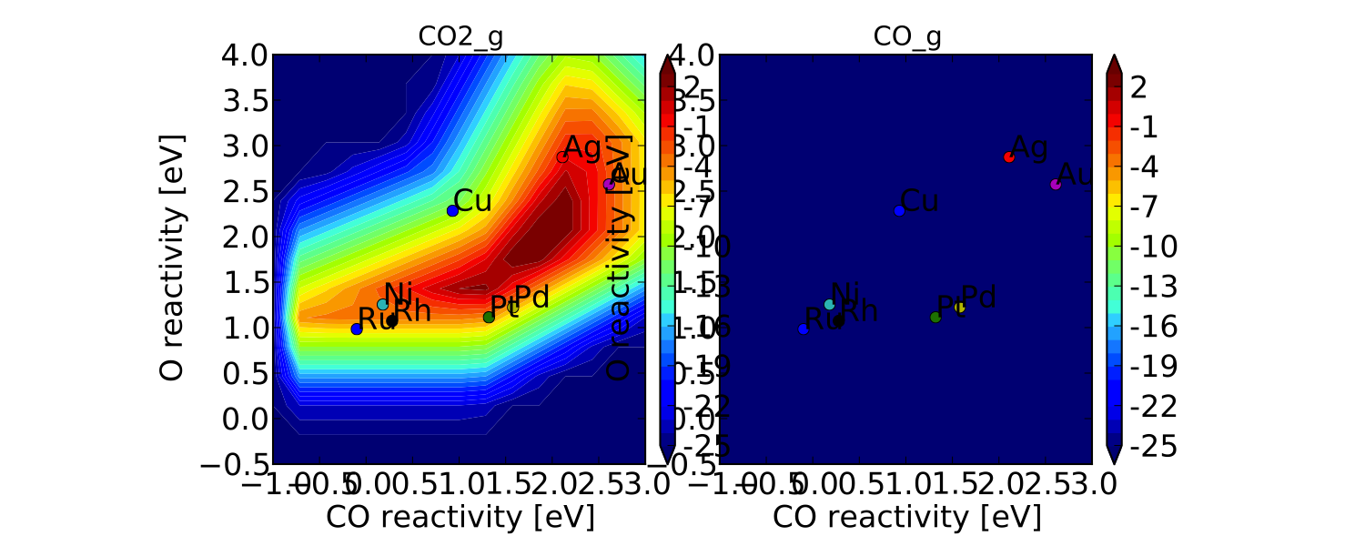
which is not very pretty. The plot on the right is showing up because the plotter says it is not empty; however, as you can see it looks pretty empty. This is happening because of numerical issues - there are some very small (<1e-50 - the tolerance) positive values for production of CO at some points in descriptor space. The quick way to get rid of this is to set a “threshold” for the plotter, so that it counts very small values as 0:

vm.descriptor_labels = ['CO reactivity [eV]', 'O reactivity [eV]']
vm.threshold = 1e-25
vm.subplots_adjust_kwargs = {'left':0.2,'right':0.8,'bottom':0.15}
vm.plot(save='pretty_production_rate.pdf')

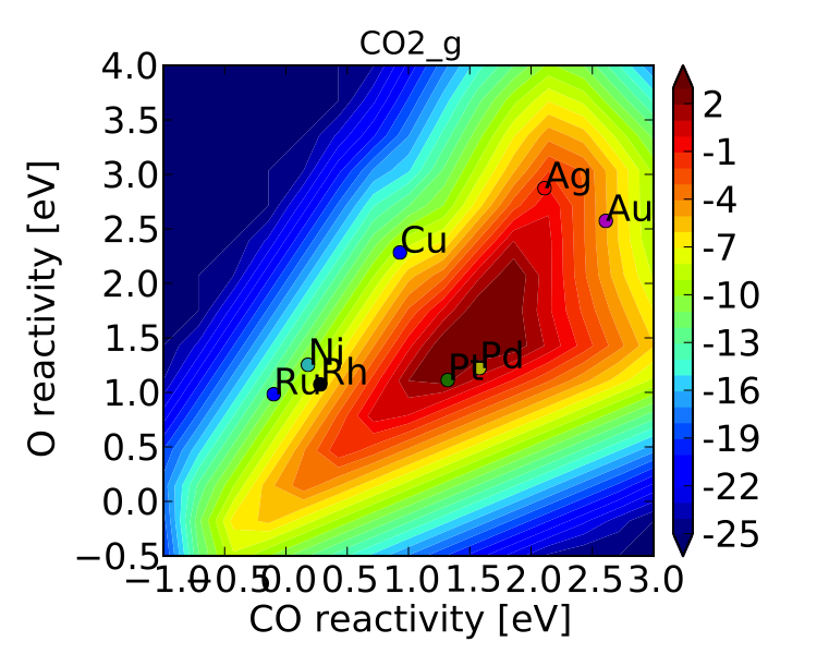
Now we get the following:

../_images/3_211_pretty_production_rate.png

The same thing can also be achieved by tightening the numerical precision/tolerance, as discussed later. When we look at the plot we see the leg going out towards Ni/Ru/Rh which, based on the previous section, we can predict will be reduced if molecular oxygen adsorption is considered. We also notice that the maximum is moved towards the nobler metals, which is roughly consistent with the findings of Falsig et. al. who show that nobler metals are more active when undercoordinated clusters are examined.

Of course in a real catalyst, there will be both (111) and (211) facets (along with lots of others, but lets focus on these two for now). We can use CatMAP to examine both facets simultaneously by adding new sites. First, we need to define the mechanisms on both sites:

rxn_expressions = [

               '\*_s + CO_g -> CO*',
               '2*_s + O2_g <-> O-O* + \*_s -> 2O*',
#               '\*_s + O2_g -> O2_s',
#               '\*_s + O2_s <-> O-O* + \*_s -> 2O*',
               'CO* +  O* <-> O-CO* + * -> CO2_g + 2*',

               '\*_t + CO_g -> CO_t',
#               '2*_t + O2_g <-> O-O* + \*_t -> 2O*',
               '\*_t + O2_g -> O2_t',
               '\*_t + O2_t <-> O-O_t + \*_t -> 2O_t',
               'CO_t +  O_t <-> O-CO_t + \*_t -> CO2_g + 2*_t',

               '\*_t + CO_s -> CO_t + \*_s',
               '\*_t + O_s -> O_t + \*_s',


                   ]

Here we use _s (or just * which is equivalent to _s) to denote step sites, and _t to denote terrace sites. We have included molecular oxygen adsorption on the terrace, but not the step since we don’t have the energetics. Diffusion between the step and terrace sites are also included, and they have no activation barrier which implies that there should be equilibrium between CO* and O* on the step/terrace. In addition to the new elementary steps, we also need to include this new “terrace site” in the species definitions:

species_definitions['s'] = {'site_names': ['211'], 'total':0.05} #define the sites
species_definitions['t'] = {'site_names': ['111'], 'total':0.95}

We also need to decide whether we want to use the (111) or (211) adsorption energies as descriptors. The proper way to do this would be to check the quality of the scaling relations and see which shows a better correlation to the parameters. However, lets just stick with the (211) sites for now.

Here we have assumed that there are 5% step sites, and 95% terrace sites. Now we can run mkm_job.py, and after a lot of fussing the model should converge. The new output looks like:

../_images/3_dual_pretty_production_rate.png

which clearly shows Pt and Pd as the best CO oxidation catalysts (as we would expect). It is a little worrying that Ag is predicted to be better than Rh, but this could be due to neglecting some mechanism (e.g. O-O-CO), neglecting zero-point and free energy contributions for adsorbates, lack of adsorbate-adsorbate interactions, or issues with the DFT input energies.

Free Energy Diagrams¶

A common way to evaluate or diagnose simpler microkinetic models is to examine the free energy diagrams that went into its creation. In the setup file, we can define any number of reaction mechanisms like the following:

rxn_mechanisms = {  # these are 1-indexed
   "steps": [1, 1, 2, 3, 3],
   "terraces": [4, 4, 5, 6, 7, 7],
}

Here we have defined two reaction mechanisms that follow the catalytic cycle of CO oxidation on steps and terraces. The array for each mechanism is composed of the 1-indexed reaction numbers as described in rxn_expressions. You can use the reverse of a given elementary step by prepending the index with a negative sign.

To actually plot the free energy diagrams, we add the following lines to mkm_job.py:

...
ma = analyze.MechanismAnalysis(model)
ma.energy_type = 'free_energy' #can also be free_energy/potential_energy
ma.include_labels = False #way too messy with labels
ma.pressure_correction = False #assume all pressures are 1 bar (so that energies are the same as from DFT)
ma.include_labels = True
fig = ma.plot(plot_variants=['Pt'], save='FED.png')
print(ma.data_dict)  # contains [energies, barriers] for each rxn_mechanism defined
...

This uses CatMAP’s built-in automatic plotter to generate free energy diagrams for your defined reaction mechanisms on all surfaces by default. For clarity, we are choosing to only plot a subset of these surfaces with the plot_variants=['Pt'] keyword argument. For electrochemical systems using ThermodynamicScaler, plot_variants instead refers to an array of voltages at which to plot free energy diagrams. The resulting plot is fairly simplistic, but feel free to generate your own nicer-looking free energy diagrams using the dictionary provided in ma.data_dict, which stores the values of free energies and barriers for each defined reaction mechanism.

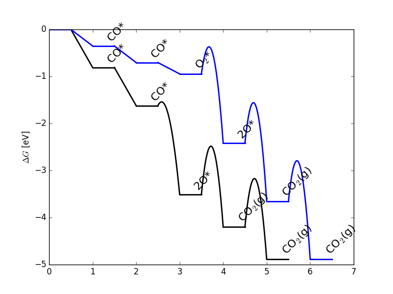
The resulting free energy diagram is a good way to quickly determine if the results of your microkinetic model match with your expectations from its free energy inputs.

Sensitivity Analyses¶

Of course the kinetic models we are building follow the golden rule of mathematical modeling: garbage in, garbage out (i.e. your model is only as good as its inputs). Even if you have the correct mechanism and active site configuration, the results will not make sense if the data in the energy tables is inaccurate. However, in order to refine these inputs it is often useful to know which ones are most important. This can be analyzed using sensitivity analyses.

Rate Control¶

The degree of rate control is a powerful concept in analyzing reaction pathways. Although many varieties exist, the version published by Stegelmann and Campbell is the most general and is implemented in the micro-kinetics module. In this definition we have:

\(X_{ij} = \frac{\mathrm{d} \log(r_i)}{\mathrm{d} (-G_j/kT)}\)

where \(X_{ij}\) is the degree of rate control matrix, \(r_i\) is the rate of production for product i, \(G_j\) is the free energy of species j, k is Boltzmann’s constant, and T is the temperature. A positive degree of rate control implies that the rate will increase by making the species more stable, while a negative degree of rate control implies the opposite.

In order to get the degree of rate control we need to add it as an output_variable in mkm_job.py:

...
mkm_file = 'CO_oxidation.mkm'
model = ReactionModel(setup_file=mkm_file)
model.output_variables += ['production_rate','rate_control']
model.run()
...

We also want to make a plot to visualize the degree of rate control:

mm = analyze.MatrixMap(model)
mm.plot_variable = 'rate_control'
mm.log_scale = False
mm.min = -2
mm.max = 2
mm.plot(save='rate_control.pdf')

The MatrixMap class is very similar to the VectorMap, except that it is designed to handle outputs which are 2-dimensional. This is true of the rate_control (and most other sensitivity analyses) since it will have a degree of rate control for each gas product/intermediate species pair. We set the min/max to -2/2 here since we know that degree of rate control is of order 1. In fact it is bounded by the number of times an intermediate appears on the same side of an elementary step. In this case that is 2, since O2* → 2O* (O* appears twice on the RHS). We could also just let the plotter decide the min/max automatically, but this is sometimes problematic due to numerical issues with rate control.

Now we can run the code. You should see that the initial guesses are proving successful for each point, but you will probably notice that the code is executing significantly slower (factor of ~16). The reason for this will be discussed later. Unlike rates/coverages, the rate control will not converge quicker with a previous solution as an initial guess. In this case it may be desirable to load in the results of a previous simulation directly like:

mkm_file = 'CO_oxidation.mkm'
#model = ReactionModel(setup_file=mkm_file)
#model.output_variables += ['production_rate','rate_control']
#model.run()

model = ReactionModel(setup_file=mkm_file.replace('mkm','log'))

In general this is a good way to re-load the results of a simulation without recalculating it. Regardless, the rate control plot looks like:

This shows us that the rate is decreased when O* or CO* are bound more strongly (depending on descriptor values). Conversely, the rate can be increased by lowering the energy of the O-CO transition state, or sometimes by binding O* more strongly at the (211) site. The effect of lowering the O-O transition-state varies depending on where the surface is in descriptor space.

While these types of analyses are useful, they should be used with caution. If the energies of other intermediates change considerably then it could result in those intermediates controlling the rate. Furthermore, as discussed by Nørskov et. al, there are underlying correlations beneath the parameters, so if one wants to optimize a catalyst these must also be considered.

Other Sensitivity Analyses¶

Similar to the degree of rate control, the degree of selectivity control can also be defined:

\(X^S_{ij} = \frac{\mathrm{d}\log(s_i)}{\mathrm{d}(-G_j/kT)}\)

where \(X^S_{ij}\) is the degree of selectivity control, and \(s_i\) is the selectivity towards species i. This can be included analogously to rate control by adding ‘selectivity_control’ to the output variables and analyzing with the MatrixMap class.

There is also the reaction order with respect to external pressures of various gasses, given mathematically by:

\(R_{ij} = \frac{\mathrm{d} \log(r_i)}{\mathrm{d} \log(pj)}\)

where \(p_j\) is the pressure of gas species j. This can also be included in the same way as rate_control and selectivity control by including “rxn_order” in the output variables.

Numerical Issues in Sensitivity Analyses¶

All sensitivity analyses implemented in the micro-kinetics module are calculated via numerical differentiation. This causes them to be very slow. Furthermore, the fact that numerical differentiation is notoriously sensitive to the “infinitesimal” number used to calculate the derivative, combined with the extreme stiffness of the sets of differential equations behind the kinetic model, can lead to issues. The two most common are:

Jacobian Errors¶

You may sometimes notice that the model will give output like:

initial_evaluation: success - initial guess at point [ 2.71, 3.36]
rootfinding_iteration_3: fail - stagnated or diverging (residual = 5.22501330063e-13)
jacobian_evaluation: fail - stagnated or diverging (residual = 5.22501330063e-13). Assuming Jacobian is 0.
initial_evaluation: success - initial guess at point [ 2.71, 3.04]

This implies that the coverages for the unperturbed parameters failed when used as an initial guess for the perturbed parameters. Given that the perturbation size is, by default, 1e-14, this should only happen if the system is extremely stiff. However, its not impossible. Usually you can figure out what you need to know even when you skip the points where the Jacobian fails, but in the case you really need it converged at every point, you can decrease the “perturbation_size” attribute of the reaction model. When specifying perturbations below 1e-14 it is probably a good idea to do this using the multiple-precision representation as:

model.perturbation_size = model._mpfloat(1e-16)

Diverging or Erroneous sensitivities¶

It is also not uncommon for the sensitivities to diverge to extremely large numbers, or just appear to be random numbers. This generally happens if the perturbation size is too small so that there is no measurable change in the values of the function. The best thing to do here is to tune the perturbation size to a slightly larger number and hope for convergence. Sometimes this does not work, in which case it might also be necessary to increase the precision and decrease the tolerance of the model by many orders of magnitude (see Refining Numerical Accuracy).

Refining Numerical Accuracy¶

A final way to refine a kinetic model is via changing the numerical parameters used for convergence, etc. A few of these parameters will be briefly discussed here:

resolution¶

The resolution determines the number of points between the min/max of the descriptor space. It can be a single number (same resolution in both directions) or a list the length of the number of descriptors. The latter case allows taking a higher resolution in one dimension vs. the other, which is useful if the descriptors have very different scales. It is also worth mentioning that a single-point calculation can be done by setting the resolution to 1. It is important to find a resolution that is fine enough to capture all the features in descriptor space, but of course higher resolution requires more time. It is also worth mentioning that if you want to refine the resolution it is good to pick a number like 2*old_resolution - 1 since this allows you to re-use all the points from the previous solution.

The CO oxidation volcano is shown below at a resolution of 29 (as opposed to 15):

../_images/3_hires_pretty_production_rate.png

It looks nicer, but doesn’t give much new insight.

decimal_precision¶

This parameter represents the numerical accuracy of the kinetic model. The solutions are found using a multiple-precision representation of numbers, so it is possible to check them to “arbitrary accuracy”. Of course the model will run slower as the decimal_precision is increased, but if the precision is not high enough then the results will not make sense. Generally a decimal_precision of ~100 is sufficient, but for complex models, or when the sensitivity analyses do not behave well, the decimal_precision sometimes needs to be increased upwards of 200-300 digits. If the solutions are correct it should be possible to increase this number arbitrarily and continue to quickly refine the precision of the solutions.

tolerance¶

The tolerance is the maximum rate which is considered 0 by the model. Thus the tolerance should be set to several orders of magnitude below the lowest rate which is relevant for the model. Usually something on the order of 1e-50 to 1e-35 is sufficient. However, when dealing with a model where the maximum rate is very low, or when trying to make sensitivity analyses more accurate, it may be necessary to decrease the tolerance to as low as 1e-decimal_precision. Similar to the decimal_precision, if the solutions are correct then it should be possible to arbitrarily decrease the tolerance (although it should never be lower than 1e-decimal_precision).

max_rootfinding_iterations¶

This determines the maximum number of times the Newton’s method rootfinding algorithm can iterate. It is generally safe to set this to a very high number, since if the algorithm begins to diverge (or even stops converging) then it will automatically exit. Usually a number around 100-300 is practical. This parameter does not affect the solutions of the model, just if/how long the model takes to converge.

max_bisections¶

This determines the number of times a distance between two points in descriptor space can be “bisected” when looking for a new solution. For example, if we know the solution at (0,0) and want the solution at (0,1) the first thing to try is using the (0,0) solution as an initial guess. If that fails, the line will be bisected, and the (0,0) solutions will be tried at (0,0.5). If this fails, then (0,0.25) is tried. This continues a maximum of max_bisections times before the module gives up. This is a “desperation” parameter since it is the best way to get a model to converge, but can be very slow. It is best to start with a value of 0-3, and then slowly increase until the algorithm can find a solution at all points. If the number goes above ~6 then it is an indication that there is something fundamentally wrong with the convergence critera (i.e. the solution oscillates) and that there is no steady-state solution.

Like max_rootfinding_iterations, max_bisections will not change the overall answers to the model, but will determine if/how long it takes to converge.